Getting Started
Resolving Exoplanets
These queries allow you to disambiguate planet names and query for planet properties.
To get a list of planet identifiers including the canonical planet name use the following query:
GET /api/v0.1/exoplanets/identifiers/?name=kepler%201b   HTTP/1.1
Host: exo.mast.stsci.edu


HTTP/1.1 200 OK
Content-Type: application/json; charset=UTF-8

{"ra": 286.80847916603085,
 "tessTCE": null,
 "planetNames": ["KIC 11446443 b",
                 "Kepler-1 b",
                 "TrES-2 b",
                 "KOI 1.01",
                 "GSC 03549-02811 b"],
 "dec": 49.316388888888895,
 "tessID": null,
 "starName": "TrES-2",
 "keplerID": 11446443,
 "keplerTCE": "TCE_1",
 "canonicalName": "TrES-2 b"}
To get properties associated with a given exoplanet canonical name use the following query:
GET /api/v0.1/exoplanets/TrES-2%20b/properties  HTTP/1.1
Host: exo.mast.stsci.edu


HTTP/1.1 200 OK
Content-Type: application/json; charset=UTF-8

{"eccentricity_ref": "O'Donovan 2006",
 "exoplanetID": 5149,
 "Tp_upper": null,
 "Fe/H_url": "http://adsabs.harvard.edu/abs/2008ApJ...677.1324T",
 "transit_time_lower": 0.0010000000474974513,
 ...}
Detrended Flux Time Series Data Queries
These services allow you to query the Data Validation Time Series data (DV Data) for Kepler and TESS. There are queries for metadata, light curves, and plots. All queries are made based on Kepler/TESS ID and transit crossing event (TCE) number.
Listing TCEs
To get a list of TCEs associated with a given Kepler or TESS ID use the following query:
GET /api/v0.1/dvdata/kepler/8394721/tces/  HTTP/1.1
Host: exo.mast.stsci.edu


HTTP/1.1 200 OK
Vary: Accept
Content-Type: application/json; charset=UTF-8

{"TCE": ["TCE_1", "TCE_3", "TCE_2", "TCE_4"]}
For TESS, the sector information will also be included in the list of TCEs:
GET /api/v0.1/dvdata/tess/388104525/tces/  HTTP/1.1
Host: exo.mast.stsci.edu


HTTP/1.1 200 OK
Vary: Accept
Content-Type: application/json; charset=UTF-8

{"TCE": ["s0001-s0003:TCE_1", "s0002-s0002:TCE_1", "s0001-s0001:TCE_1", "s0003-s0003:TCE_1",
"s0001-s0002:TCE_1", "s0007-s0007:TCE_1", "s0004-s0004:TCE_1"]}
Metadata queries
There are two metadata queries. To get the data column names, types, and descriptions for DV Data queries, use the following query:
GET /api/v0.1/dvdata/tess/info  HTTP/1.1
Host: exo.mast.stsci.edu

HTTP/1.1 200 OK
Content-Length: 12694
Content-Type: application/json; charset=UTF-8

{"DV Data Table Description": [
    {"description": "unique tess target identifier",
     "colname": "TICID",
     "datatype": "int"},
    {"description": "name of extension",
     "colname": "EXTNAME",
     "datatype": "varchar(10)"}, ...
To get metadata about a specific Kepler or TESS target with or without associated TCE use the following query (if the TCE is ommitted, the TCE specific metatdata will simply not be returned):
GET /api/v0.1/dvdata/kepler/8394721/info/?tce=1 HTTP/1.1
Host: exo.mast.stsci.edu

HTTP/1.1 200 OK
Vary: Accept
Content-Type: application/json; charset=UTF-8

{"DV Data Header": {DATE_OBS: "2009-05-13 00:01:07.137000",
                    PRADIUS; 7.414486640355018,
                    ...},
 "DV Primary Header": {NEXTEND: 6,
                       OBJECT: "KIC 8394721",
                       AV: 0.398,
                       ...} }
Note that TESS info queries with TCE require the sector be provided, otherwise they will return with a 400 status error. The sector can be provided as a single number (which represents a single sector) or as the TESS sector range notation (eg, s0001-s0002). See the example below:
GET /api/v0.1/dvdata/tess/388104525/info/?tce=1§or=s0003-s0003 HTTP/1.1
Host: exo.mast.stsci.edu
HTTP/1.1 200 OK
Vary: Accept
Content-Type: application/json; charset=UTF-8
{"DV Data Header": {DATE_OBS: "2018-11-15 11:25:52.487000",
TICID; 388104525,
...},
"DV Primary Header": {NEXTEND: 6,
OBJECT: "TIC 388104525",
...} }
Data queries
To get the detrended lightcurve data table for a given Kepler/TESS ID and TCE use the following query:
GET /api/v0.1/dvdata/kepler/8394721/table/?tce=2 HTTP/1.1
Host: exo.mast.stsci.edu

HTTP/1.1 200 OK
Vary: Accept
Content-Type: application/json; charset=UTF-8

{"fields":[{colname: "KEPLERID",
            datatype: "int",
            description: "unique Kepler target identifier"},
           ...],
 "data": [{'EXTNAME': 'TCE_2',
           'MODEL_WHITE': -0.02279440499842167,
           'PHASE': 8.375410079956055,
           'LC_INIT_ERR': 0.00019099553173873574,
           'LC_INIT': 0.0006834766245447099,
           'LC_WHITE': 2.559422492980957,
           'CADENCENO': 1105,
           'LC_DETREND': 0.0006834766245447099,
           'MODEL_INIT': 0.0,
           'TIMECORR': -0.0007000599289312959,
           'KEPLERID': 8394721,
           'TIME': 131.51169387994014},
          ...]}
Note that TESS data table queries require both the TCE and Sector be provided, otherwise they will return with a 400 status error. For a list of sector/tce options, use the /tces endpoint described above. The sector can be provided as a single number (which represents a single sector) or as the TESS sector range notation (eg, s0001-s0002). See the example below:
GET /api/v0.1/dvdata/tess/388104525/table/?tce=1§or=s0003-s0003 HTTP/1.1
Host: exo.mast.stsci.edu
HTTP/1.1 200 OK
Vary: Accept
Content-Type: application/json; charset=UTF-8
{"fields":[{colname: "TIME",
datatype: "float",
description: "column title: data time stamps"},
...],
"data": [{'EXTNAME': 'TCE_1',
'MODEL_WHITE': -0.02279440499842167,
'PHASE': 8.375410079956055,
'LC_INIT_ERR': 0.00019099553173873574,
'LC_INIT': 0.0006834766245447099,
'LC_WHITE': 2.559422492980957,
'CADENCENO': 1105,
'LC_DETREND': 0.0006834766245447099,
'MODEL_INIT': 0.0,
'TIMECORR': -0.0007000599289312959,
'TESSID': 388104525,
'TIME': 131.51169387994014,
'SECTORS': 's0003-s0003'},
...]}
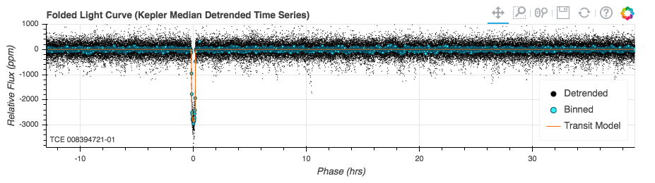
Instead of getting the light curve as a data table, you can also directly query for phase folded plots of the light curve. The plots can be returned as html that can be directly viewed in a browser, or as embeddable componants suitable for inclusion in a larger website. You can request a simple phase folded plot for viewing in the browser with the following query:
GET /api/v0.1/dvdata/kepler/8394721/phaseplot/?tce=2 HTTP/1.1
Host: exo.mast.stsci.edu

HTTP/1.1 200 OK
Content-Type text/html; charset=UTF-8

<!DOCTYPE html>
<html lang="en">
  <head>
     <meta charset="utf-8">
     <title>Phased Light Curve</title>

     <link rel="s...
To request the plot as embeddable elements simply add the embed argument:
GET /api/v0.1/dvdata/kepler/8394721/phaseplot/?tce=2&embed HTTP/1.1
Host: exo.mast.stsci.edu

HTTP/1.1 200 OK
Vary: Accept
Content-Type: text/javascript

{resources: {js:   "\\n<script type=\\"text/ja...,
             css:"\\n<style>\\n /* BEGIN... },
 script: "\\n<script type-\\"text/ja...,
 div: "\\n<div class=\\"bk-root\\"...}
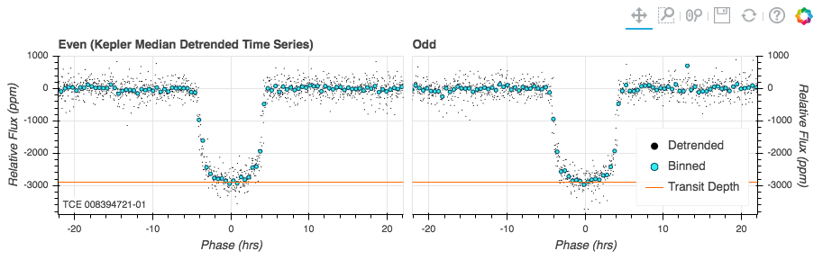
You can also request the plot split into even and odd phases:
GET /api/v0.1/dvdata/kepler/8394721/phaseplot/?tce=2&splitphase HTTP/1.1
Host: exo.mast.stsci.edu

HTTP/1.1 200 OK
Content-Type text/html; charset=UTF-8

<!DOCTYPE html>
<html lang="en">
  <head>
     <meta charset="utf-8">
     <title>Phased Light Curve</title>

     <link rel="s...
The phase plot can be displayed in a Jupyter Notebook as in the following example:
>>> import requests
>>> from IPython.display import display, HTML
>>> spectra_plot = requests.get("https://exo.mast.stsci.edu/api/v0.1/dvdata/kepler/6278762/phaseplot/?tce=TCE_1")
>>> display(HTML(str(spectra_plot.content.decode('utf-8'))))
Like the table/ and tces/ endpoints, the phaseplot/ endpoint for TESS requires both the TCE and Sector be provided, otherwise they will return with a 400 status error.
Exoplanet Spectra Queries
These queries allow you to access information about the spectra of a specific exoplanet.
This query allows you to get a list of spectra files associated with a given planet:
GET /api/v0.1/spectra/Hat-P-11%20b/filelist/   HTTP/1.1
Host: exo.mast.stsci.edu


HTTP/1.1 200 OK
Vary: Accept
Content-Type: application/json; charset=UTF-8

{"filename": ["HAT-P-11b_transmission_Fraine2014.txt"]}
To download a particular spectra file use the following query:
GET /api/v0.1/spectra/Hat-P-11%20b/file/HAT-P-11b_transmission_Fraine2014.txt  HTTP/1.1
Host: exo.mast.stsci.edu

HTTP/1.1 200 OK
Vary: Accept

# HAT-P-11b transmission spectrum
# This file contains:
# WFC3 G141 - GO 12449 - Fraine, et al., 2014, Nature
# Data history:
# Converted from: Fraine, et al., 2014, Nature
# ----------------------------------------------------------------------------------------
# Wavelength (microns)  Delta Wavelength (microns)  (Rp/Rs)^2   (Rp/Rs)^2 +/-uncertainty
# ----------------------------------------------------------------------------------------
         1.1530000    0.00950003   0.00350200   0.00004000
         1.1720001    0.00950003   0.00340700   0.00004700
         1.1900001    0.00950003   0.00342100   0.00004600
         1.2090000    0.00950003   0.00344500   0.00003800
         1.2280000    0.00950003   0.00335000   0.00004100
         1.2470000    0.00950003   0.00337700   0.00003800
         1.2660000    0.00950003   0.00338000   0.00004500
         1.2840000    0.00950003   0.00345700   0.00004000
         1.3030000    0.00950003   0.00343600   0.00003500
         1.3220000    0.00950003   0.00344800   0.00003900
         1.3410000    0.00950003   0.00347600   0.00004300
         1.3600000    0.00950003   0.00353600   0.00004400
         1.3789999    0.00950003   0.00349900   0.00004600
         1.3970000    0.00950003   0.00349800   0.00004000
         1.4160000    0.00950003   0.00352400   0.00004100
         1.4349999    0.00950003   0.00359100   0.00004400
         1.4540000    0.00950003   0.00352400   0.00004300
         1.4730000    0.00950003   0.00352000   0.00003900
         1.4920000    0.00950003   0.00344700   0.00003900
         1.5100000    0.00950003   0.00334400   0.00004500
         1.5290000    0.00950003   0.00351300   0.00004100
         1.5480000    0.00950003   0.00347100   0.00005000
         1.5670000    0.00950003   0.00343800   0.00004900
         1.5860000    0.00950003   0.00341400   0.00005300
         1.6040000    0.00950003   0.00338300   0.00004500
         1.6230000    0.00950003   0.00341500   0.00003800
         1.6420000    0.00950003   0.00348000   0.00004800
         1.6610000    0.00950003   0.00349800   0.00006000
         1.6799999    0.00950003   0.00337600   0.00007400
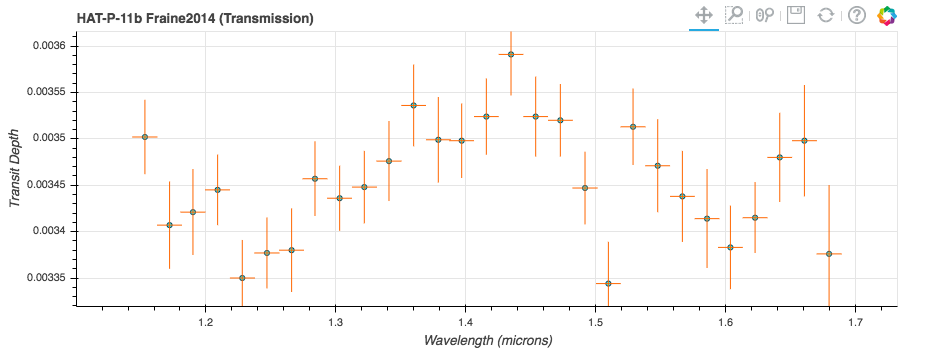
Instead of getting the spectra information as a data file, you can also directly query for spectra plots. The plot can be returned as html that can be directly viewed in a browser, or as embeddable componants suitable for inclusion in a larger website. You can request a spectra plot for viewing in the browser with the following query:
GET /api/v0.1/spectra/Hat-P-11%20b/plot/ HTTP/1.1
Host: exo.mast.stsci.edu

HTTP/1.1 200 OK
Content-Type text/html; charset=UTF-8

<!DOCTYPE html>
<html lang="en">
  <head>
     <meta charset="utf-8">
     <title>Time Series</title>

     <link rel="s...
The spectra plot can be displayed in a Jupyter Notebook as in the following example:
>>> import requests
>>> from IPython.display import display, HTML
>>> spectra_plot = requests.get("https://exo.mast.stsci.edu/api/v0.1/spectra/Hat-P-11%20b/plot/")
>>> display(HTML(str(spectra_plot.content.decode('utf-8'))))